Lecture 17: Tensors and tensor decompositions¶

Recap of the previous lecture¶

Matrix functions (matrix exponentials, matrix sign function, Schur-Parlett algorithm, ...)
Matrix equations

Today lecture¶

Tensor decompositions and applications

Tensors¶

By tensor we imply a multidimensional array:

$$ A(i_1, \dots, i_d), \quad 1\leq i_k\leq n_k, $$

where $d$ is called dimension, $n_k$ - mode size. This is standard definition in applied mathematics community. For details see [1], [2], [3].

$d=2$ (matrices) $\Rightarrow$ classic theory (SVD, LU, QR, $\dots$)
$d\geq 3$ (tensors) $\Rightarrow$ under development. Generalization of standard matrix results is not straightforward.

Picture is taken from this presentation

More formal definition¶

Tensor is a multilinear form. When you fix the basis, you get a $d$-dimensional table.

Curse of dimensionality¶

The problem with multidimensional data is that number of parameters grows exponentially with $d$:

$$ \text{storage} = n^d. $$ For instance, for $n=2$ and $d=500$ $$ n^d = 2^{500} \gg 10^{83} - \text{ number of atoms in the Universe} $$

Why do we care? It seems that we are living in the 3D World :)

Applications¶

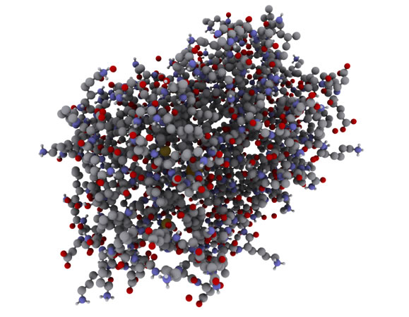
Quantum chemistry¶

Stationary Schroedinger equation for system with $N_{el}$ electrons

$$ \hat H \Psi = E \Psi, $$

where

$$ \Psi = \Psi(\{{\bf r_1},\sigma_1\},\dots, \{{\bf r_{N_{el}}},\sigma_{N_{el}}\}) $$

3$N_{el}$ spatial variables and $N_{el}$ spin variables.

Drug and material design
Predicting physical experiments

Uncertainty quantification¶

Example: oil reservoir modeling. Model may depend on parameters $p_1,\dots,p_d$ (like measured experimentally procity or temperature) with uncertainty

$$ u = u(t,{\bf r},\,{p_1,\dots,p_d}) $$

And many more¶

Signal processing
Recommender systems
Neural networks
Language models
Financial mathematics
...

Working with many dimensions¶

How to work with high-dimensional functions?

Monte-Carlo: class of methods based on random sampling. Convergence issues
Sparse grids: special types of grids with small number of grid points. Strong regularity conditions
Best N-term approximation : sparse expansions in certain basis.
Promising approach based on tensor decompositions

Tensor decompositions¶

2D¶

Skeleton decomposition: $$ A = UV^T $$ or elementwise: $$ a_{ij} = \sum_{\alpha=1}^r u_{i\alpha} v_{j\alpha} $$ leads us to the idea of separation of variables.

Properties:

Not unique: $A = U V^T = UBB^{-1}V^T = \tilde U \tilde V^T$
Can be calculated in a stable way by SVD

Canonical decomposition¶

The most straightforward way to generize separation of variables to many dimensions is the canonical decomposition: (CP/CANDECOMP/PARAFAC)

$$ a_{ijk} = \sum_{\alpha=1}^r u_{i\alpha} v_{j\alpha} w_{k\alpha} $$

minimal possible $r$ is called the canonical rank. Matrices $U$, $V$ and $W$ are called canonical factors. This decomposition was proposed in 1927 by Hitchcock, link.

Properties:

For a $d$ dimensional tensor memory is $nrd$
Unique under mild conditions
Set of tensors with rank$\leq r$ is not closed (by contrast to matrices):
$a_{ijk} = i+j+k$, $\text{rank}(A) = 3$, but

$$a^\epsilon_{ijk} = \frac{(1+\epsilon i)(1+\epsilon j)(1+\epsilon k) - 1}{\epsilon}\to i+j+k=a_{ijk},\quad \epsilon\to 0 $$

and $\text{rank}(A^{\epsilon}) = 2$
No stable algorithms to compute best rank-$r$ approximation

Alternating Least Squares algorithm¶

Intialize random $U,V,W$
fix $V,W$, solve least squares for $U$
fix $U,W$, solve least squares for $V$
fix $U,V$, solve least squares for $W$
go to 2.

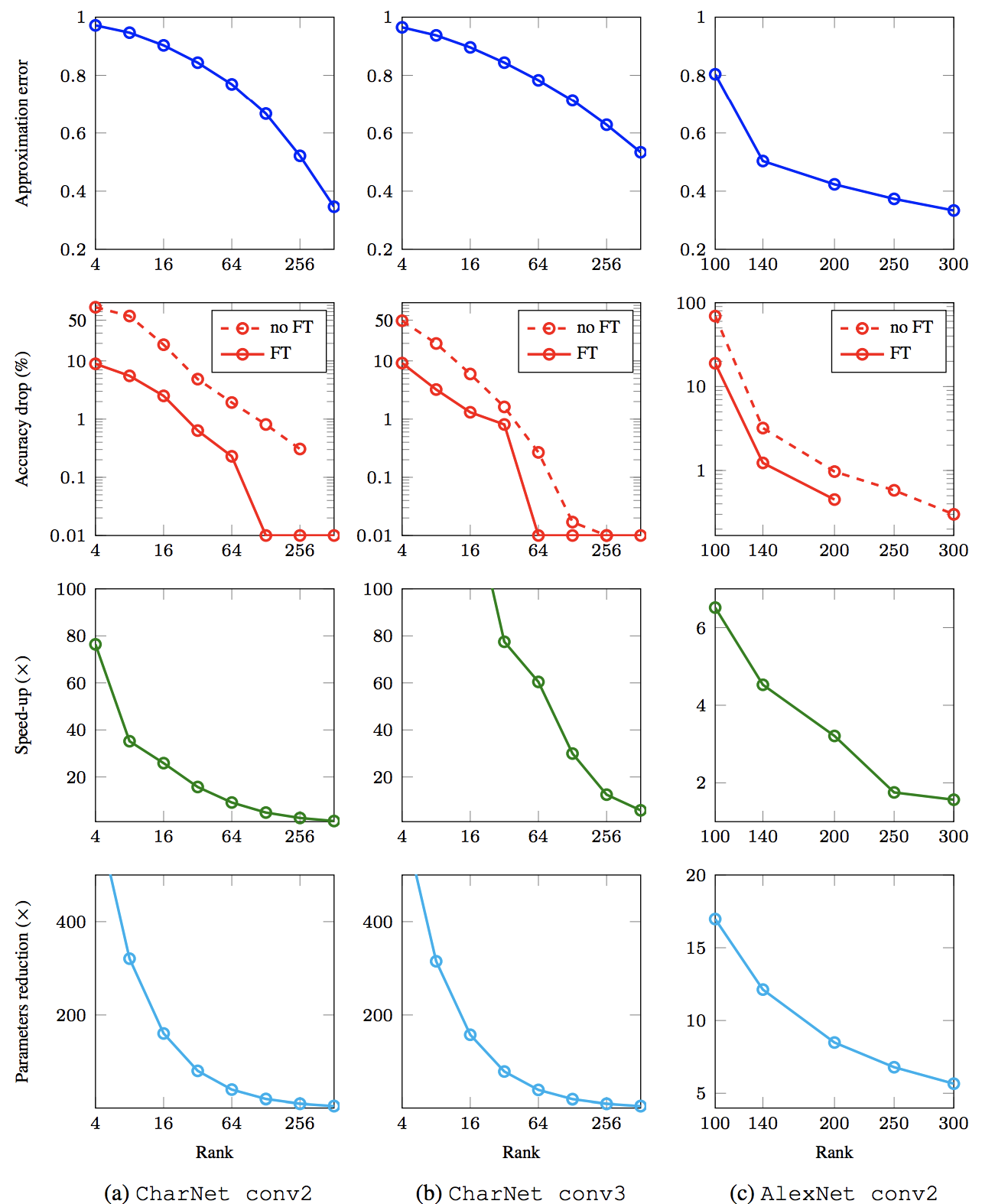
DNN compression (Lebedev, et. al 2015)¶

Convolution is represented as 4D tensor
Apply CP decomposition to this tensor
Apply one-by-one convolutions with smaller kernels given by CP decomposition
Fine tune such model

In [1]:

import tensorly as tl
import tensorly.decomposition as tldec
import numpy as np
import matplotlib.pyplot as plt
%matplotlib inline

tensor = tl.tensor(np.arange(24).reshape((3, 4, 2)))
# tensor = tl.random.cp_tensor(shape=(3,3,3), rank=3, full=True)
print(tensor)
rank_range = [1, 2, 3, 4, 5, 6]
error_rec = []
for r in rank_range:
    factors = tldec.parafac(tensor, rank=r)
    error_rec.append(np.linalg.norm(tl.kruskal_to_tensor(factors) - tensor))
plt.semilogy(rank_range, error_rec)
plt.xlabel("CP rank")
plt.ylabel("Approximation error")

Using numpy backend.

[[[ 0.  1.]
  [ 2.  3.]
  [ 4.  5.]
  [ 6.  7.]]

 [[ 8.  9.]
  [10. 11.]
  [12. 13.]
  [14. 15.]]

 [[16. 17.]
  [18. 19.]
  [20. 21.]
  [22. 23.]]]

Out[1]:

Text(0,0.5,'Approximation error')

Tucker decomposition¶

Next attempt is the decomposition proposed by (Tucker, 1963) in Psychometrika:

$$ a_{ijk} = \sum_{\alpha_1,\alpha_2,\alpha_3=1}^{r_1,r_2,r_3}g_{\alpha_1\alpha_2\alpha_3} u_{i\alpha_1} v_{j\alpha_2} w_{k\alpha_3}. $$

Here we have several different ranks. Minimal possible $r_1,r_2,r_3$ are called Tucker ranks.

Properties:

For a $d$ dimensional tensor memory is $r^d$ $+ nrd$. Still curse of dimensionality
Stable SVD-based algorithm:
1. $U =$ principal components of the unfolding A.reshape(n1, n2*n3)
2. $V =$ principal components of the unfolding A.transpose([1,0,2]).reshape(n2, n1*n3)
3. $W =$ principal components of the unfolding A.transpose([2,0,1]).reshape(n3, n1*n2)
4. $g_{\alpha_1\alpha_2\alpha_3} = \sum_{i,j,k=1}^{n_1,n_2,n_3} a_{ijk} u_{i\alpha_1} v_{j\alpha_2} w_{k\alpha_3}$.

In [2]:

tensor = tl.tensor(np.arange(24).reshape((3, 4, 2)))
core, factors = tldec.tucker(tensor, ranks=[3, 4, 2])
print("Shape of core = {}".format(core.shape))
for f in factors:
    print("Shape of factors = {}".format(f.shape))
print("Approximation error = {}".format(np.linalg.norm(tensor - tl.tucker_to_tensor(core, factors))))

Shape of core = (3, 4, 2)
Shape of factors = (3, 3)
Shape of factors = (4, 4)
Shape of factors = (2, 2)
Approximation error = 3.181718859384126e-14

Application in recommender systems (Frolov, Oseledets 2016)¶

Represent User-Item matrix as binary User-Item-Rating tensor
After Tucker decomposition of this tensor we have three factors
Two of them represent projections on the space of ratings and space of items
This approach takes into account negative feedback to items from some users

CP and Tucker decompositions implementations¶

Matlab: Tensorlab and Tensor Toolbox
Python: TensorLy and Scikit-tensor

Tensor Train decomposition¶

Calculation of the canonical decomposition is unstable
Tucker decomposition suffers from the curse of dimensionality

Tensor Train (TT) decomposition (Oseledets, Tyrtyshnikov 2009 and Oseledets, 2011) is both stable and contains linear in $d$ number of parameters:

$$ a_{i_1 i_2 \dots i_d} = \sum_{\alpha_1,\dots,\alpha_{d-1}} g_{i_1\alpha_1} g_{\alpha_1 i_2\alpha_2}\dots g_{\alpha_{d-2} i_{d-1}\alpha_{d-1}} g_{\alpha_{d-1} i_{d}} $$

or in the matrix form

$$ a_{i_1 i_2 \dots i_d} = G_1 (i_1)G_2 (i_2)\dots G_d(i_d) $$

The storage is $\mathcal{O}(dnr^2)$
Stable TT-SVD algorithm

Example $$a_{i_1\dots i_d} = i_1 + \dots + i_d$$ Canonical rank is $d$. At the same time TT-ranks are $2$: $$ i_1 + \dots + i_d = \begin{pmatrix} i_1 & 1 \end{pmatrix} \begin{pmatrix} 1 & 0 \\ i_2 & 1 \end{pmatrix} \dots \begin{pmatrix} 1 & 0 \\ i_{d-1} & 1 \end{pmatrix} \begin{pmatrix} 1 \\ i_d \end{pmatrix} $$

Implementations¶

Matlab: TT Toolbox
Python: ttpy
TensorFlow: t3f

Using TT in riemannien optimization (example is from t3f examples)¶

Given some TT tensor $A$ with large tt-ranks
We would like to find a tensor $X$ (with small prescribed tt-ranks $r$) which is closest to $A$ (in the sense of Frobenius norm): \begin{equation*} \begin{aligned} & \underset{X}{\text{minimize}} & & \frac{1}{2}\|X - A\|_F^2 \\ & \text{subject to} & & \text{tt_rank}(X) = r \end{aligned} \end{equation*}
It is known that the set of TT tensors with elementwise fixed TT ranks forms a manifold.
Thus we can solve this problem using the so called Riemannian gradient descent.

Riemannian gradient descent¶

Given some functional $F$ on a manifold $\mathcal{M}$ Riemannian gradient descent is defined as

$$\hat{x}_{k+1} = x_{k} - \alpha P_{T_{x_k}\mathcal{M}} \nabla F(x_k),$$

$$x_{k+1} = \mathcal{R}(\hat{x}_{k+1})$$

with $P_{T_{x_k}\mathcal{M}}$ being the projection onto the tangent space of $\mathcal{M}$ at the point $x_k$ and $\mathcal{R}$ being a retraction - an operation which projects points to the manifold, and $\alpha$ is the learning rate.

We can implement this in t3f using the t3f.riemannian module. As a retraction it is convenient to use the rounding method (t3f.round).

In [3]:

import t3f
import tensorflow as tf
tf.set_random_seed(0)
np.random.seed(0)
sess = tf.InteractiveSession()

# Initialize A randomly, with large tt-ranks
shape = 10 * [2]
init_A = t3f.random_tensor(shape, tt_rank=16)
A = t3f.get_variable('A', initializer=init_A, trainable=False)

# Create an X variable and compute the gradient of the functional. Note that it is simply X - A.

init_X = t3f.random_tensor(shape, tt_rank=2)
X = t3f.get_variable('X', initializer=init_X)

gradF = X - A

In [4]:

# Let us compute the projection of the gradient onto the tangent space at X
riemannian_grad = t3f.riemannian.project(gradF, X)

# Compute the update by subtracting the Riemannian gradient
# and retracting back to the manifold
alpha = 1.0

train_step = t3f.assign(X, t3f.round(X - alpha * riemannian_grad, max_tt_rank=2))

# let us also compute the value of the functional
# to see if it is decreasing
F = 0.5 * t3f.frobenius_norm_squared(X - A)

In [5]:

sess.run(tf.global_variables_initializer())

log = []
for i in range(100):
    F_v, _ = sess.run([F, train_step.op])
    if i % 10 == 0:
        print (F_v)
    log.append(F_v)

It is intructive to compare the obtained result with the quasioptimum delivered by the TT-round procedure.

In [6]:

quasi_sol = t3f.round(A, max_tt_rank=2)

val = sess.run(0.5 * t3f.frobenius_norm_squared(quasi_sol - A))
print (val)

52.40742

We see that the value is slightly bigger than the exact minimum, but TT-round is faster and cheaper to compute, so it is often used in practice.

In [7]:

plt.semilogy(log, label='Riemannian gradient descent')
plt.axhline(y=val, lw=1, ls='--', color='gray', label='TT-round(A)')
plt.xlabel('Iteration')
plt.ylabel('Value of the functional')
plt.legend()

Out[7]:

<matplotlib.legend.Legend at 0xd261fa4a8>

Exponential machines (Novikov et al 2017)¶

Linear model depends on vector

$$ \hat{y}_l(x) = \langle w, x \rangle + b$$

Exponential machine depends on tensor $W$

$$\hat{y}_{expm}(x) = \sum_{i_1 = 0}^1 \ldots \sum_{i_d = 0}^1 W_{i_1, \ldots, i_d} \prod_{k=1}^d x_k^{i_k}$$

Represent tensor $W$ in TT-format and control TT-rank
Learning of this model is loss minimization with constraint on the tensor rank - riemannien optimization again

Quantized Tensor Train¶

Consider a 1D array $a_k = f(x_k)$, $k=1,\dots,2^d$ where $f$ is some 1D function calculated on grid points $x_k$.

Let $$k = {2^{d-1} i_1 + 2^{d-2} i_2 + \dots + 2^0 i_{d}}\quad i_1,\dots,i_d = 0,1 $$ be binary representation of $k$, then

$$ a_k = a_{2^{d-1} i_1 + 2^{d-2} i_2 + \dots + 2^0 i_{d}} \equiv \tilde a_{i_1,\dots,i_d}, $$

where $\tilde a$ is nothing, but a reshaped tensor $a$. TT decomposition of $\tilde a$ is called Quantized Tensor Train (QTT) decomposition.

Interesting fact is that the QTT decomposition has relation to wavelets, more details see here.

Contains $\mathcal{O}(\log n r^2)$ elements!

Cross approximation method¶

If decomposition of a tensor is given, then there is no problem to do basic operations fast.
However, the question is if it is possible to find decomposition taking into account that typically tensors even can not be stored.
Cross approximation method allows to find the decomposition using only few of its elements (more details in the blackboard).

Tensor networks¶

Universal way for writing tensor decompositions
Can be interpreted as special neural network architecture
Some theoretical results on DNN expressive power can be derived with tensor network framework, see an example here
Tntorch combines tensor networks and PyTorch
More details see here and here

Summary¶

Tensor decompositions - useful tool to work with multidimensional data
Canonical, Tucker, TT, QTT decompositions
Cross approximation

Next week¶

Exam: Monday and Tuesday